Last Modified: 2023-Jun-29
Remember to right click->"open image in new tab" for small images
Índice
Voronoi representation
From the previous work, I conclude the algorithm for path solving was highly dependant on the cells graph. We need to connect each cell with all the of neighbouring cells, as with the sphere of influence moving throughout this cell graph is seen as us moving farther from the first cell and closer to the second one.
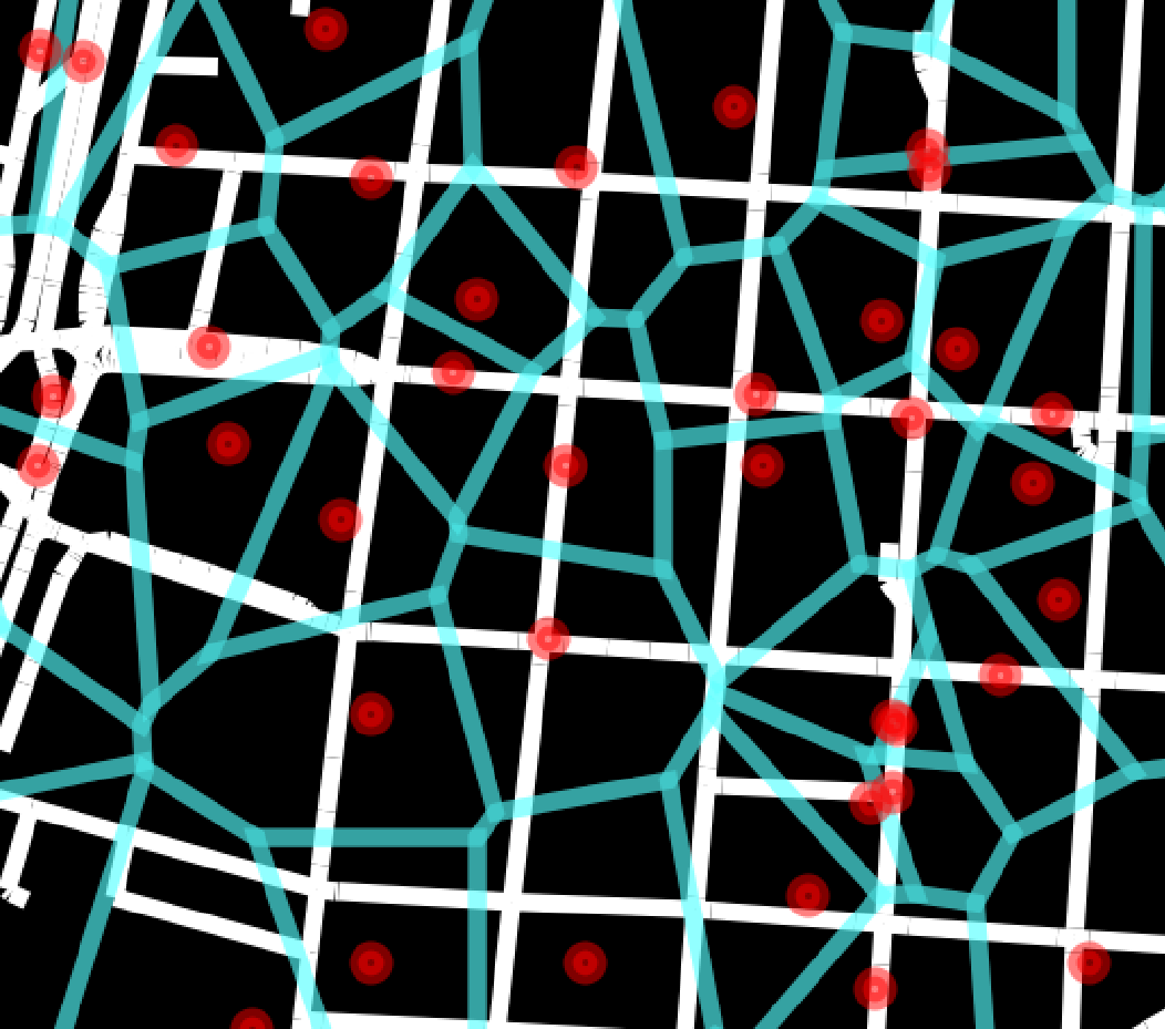
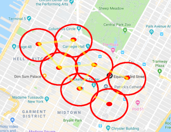
The Voronoi representation allows us to make a graph where each cell has an edge to each neighbouring cell. See image below, edges in gray, cells (red dots).
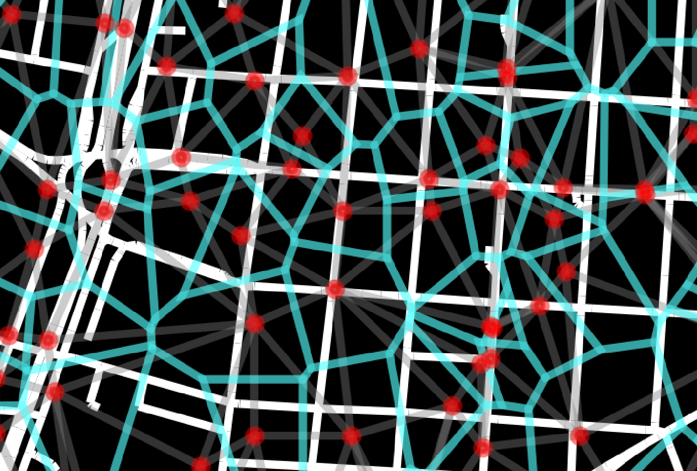
On the left, the voronoi regions(in blue) and their cells (red dots), on the right, in transparent gray the resulting graph’s edges
Many works also use Voronoi for modelling this kind of networks
Considerations
- 👍 I’m using plain Voronoi, not having into consideration the cell’s power,
rangefield in opencellid database (unreliable field) - 👍 Being inside a region of a cell means that most likely your phone will be connected to that tower cell
- 👎 Voronoi regions cover all of the map, there’s not any spot with no coverage, not true for remote places
- 👍👍👍👍👍👍👍 It looks good
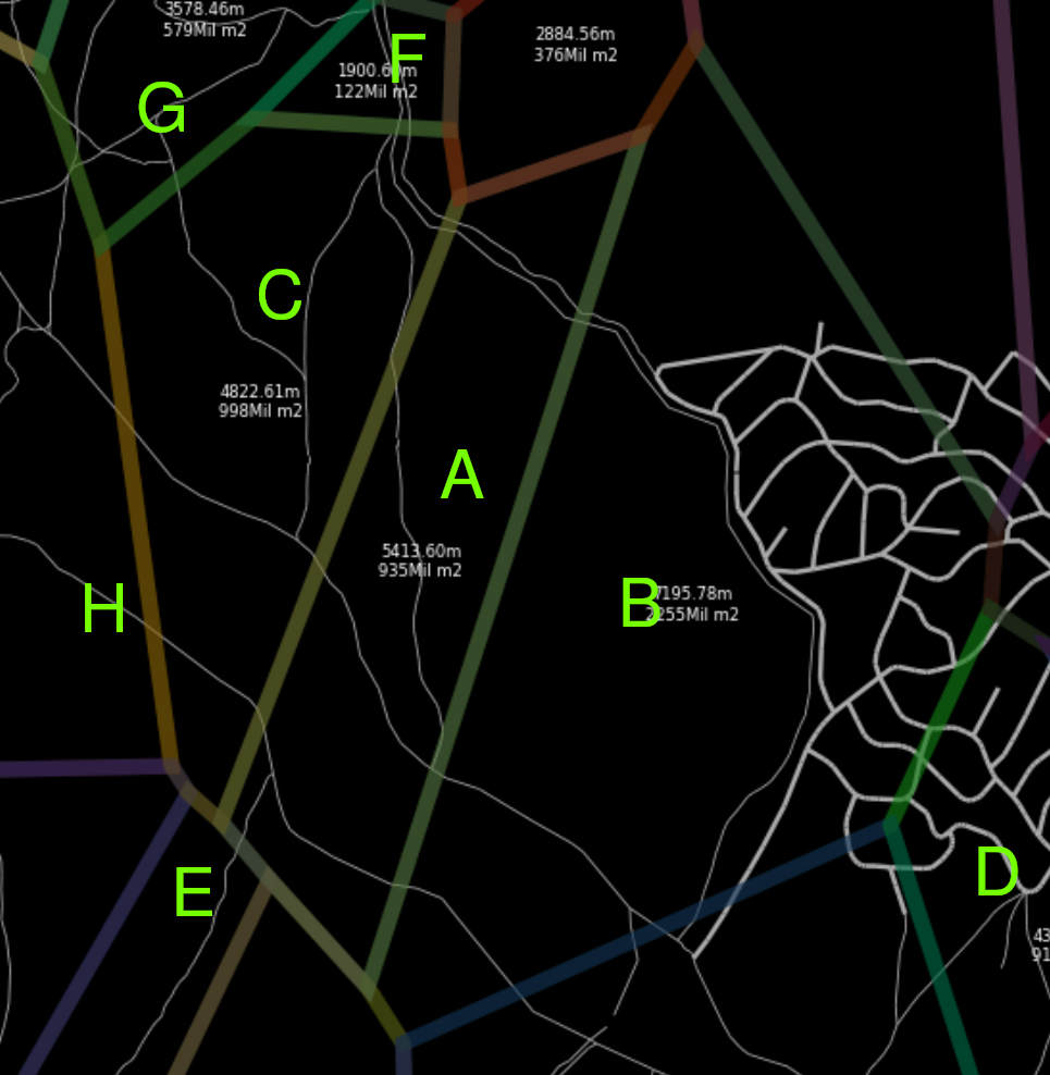
Inside each V. region, the perimeter in meters and area in (area [m^2])/1000, and width of the ways by their kind (thicker primary,thinnest dirt ones)
Ok, looks cool what about the Algorithm
At first glance, using the same algorithm as before shortest path in cell graph gives us the same kind of problems as it did before.
- It seems pointless to check the roads inside a cell’s range more than one time, roads don’t move.
- The shortest path in the cell’s graph has zero value, we might as well pick a path with S shape and try to find a valid road path which satisfies reachability The shortest path in the cell’s graph would make sense if the landscape of the town was a grid or we have the guarantee a neighbouring cell has a road path which connects the roads under their coverage.
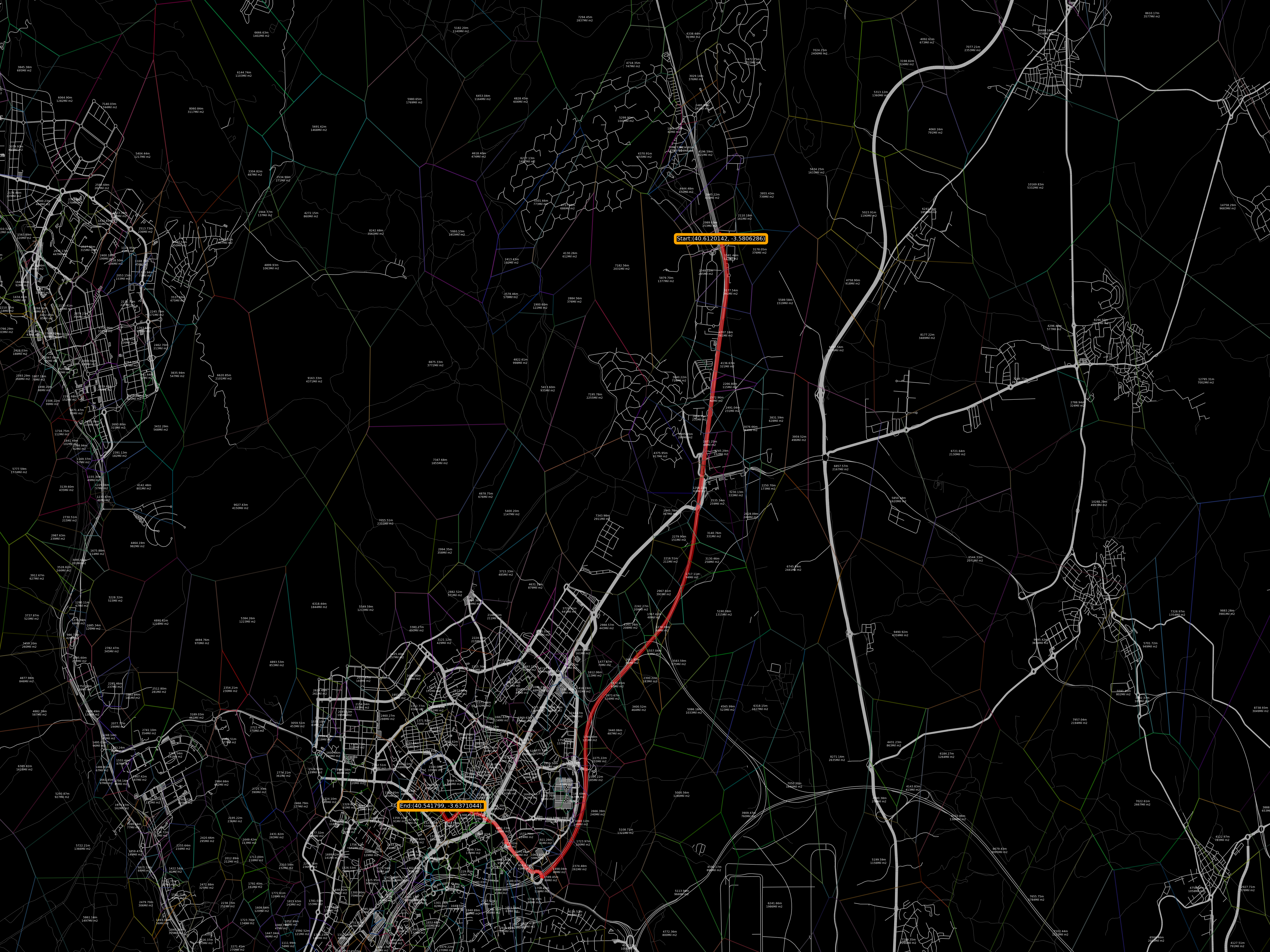
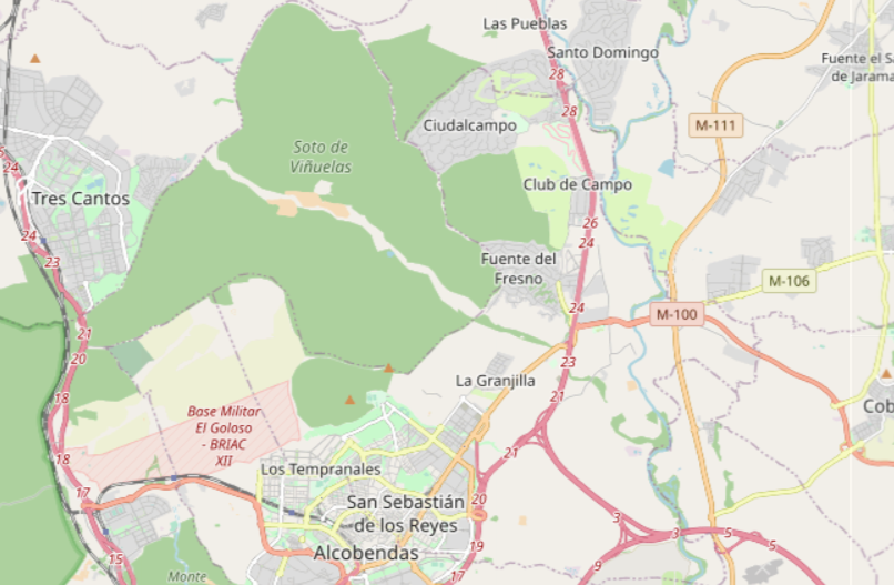
On the left, Manhattan, every road under every cell is reachable, on the right, Fuente de Fresno, Madrid, on which I will explain the new algorithm.
Using the old algorithm is just too slow, the cell’s graph give little information about how we can move from one cell to another by road.
Addressing both concerns, I came with this solution
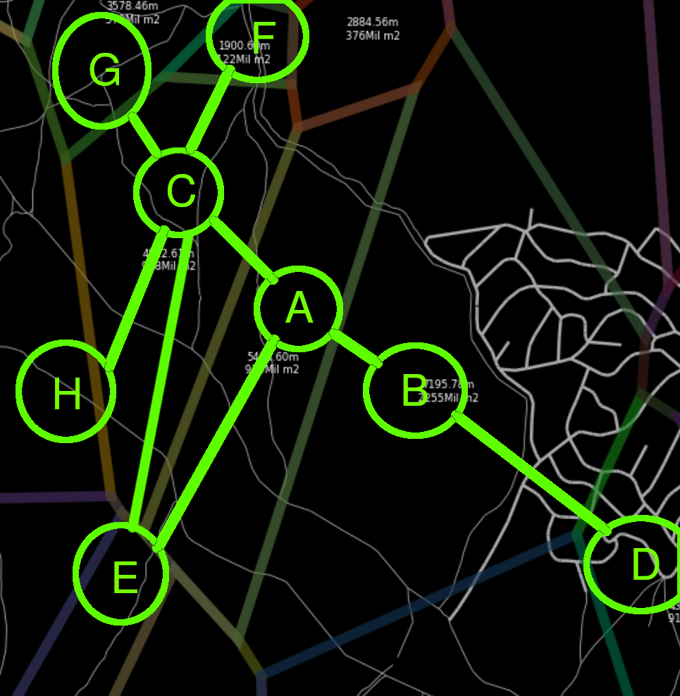
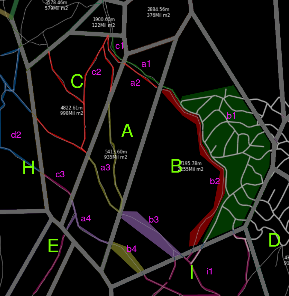
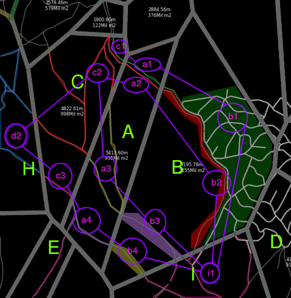
A voronoi region A contains 1 or more unreachable roads, each set of roads A1, A2, A3, A4 is connected or not to a neighbouring cell’s set of roads A1 - C1, A2 - C2, A3 - C2, , A4, C3.
Hence, we can define a graph which only contains these sets of roads with the property that if the node Xi can reach Xj, hence, every road point from Xi can reach Xj.
The path solving would be performed like this
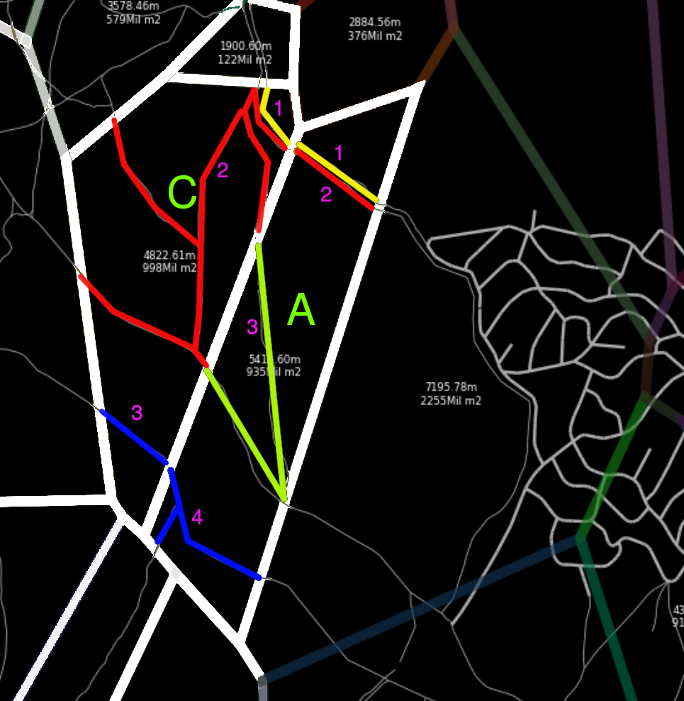
For example, see P1 and P2. They are under the same cell: A, with the old algorithm we would end the search in the cell’s graph because the closer base station to P1 is the same as P2.
Using this new algorithm:
- From
P1we get the set of roads which contains it ->A3 -
From
P2we get the set of roads which contains it ->A4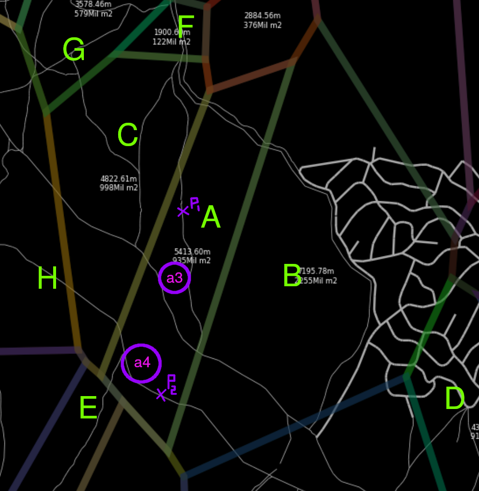
-
We obtain a path between
A3andA4. i.e.(Using A*)A3,C2,D2,C3,A4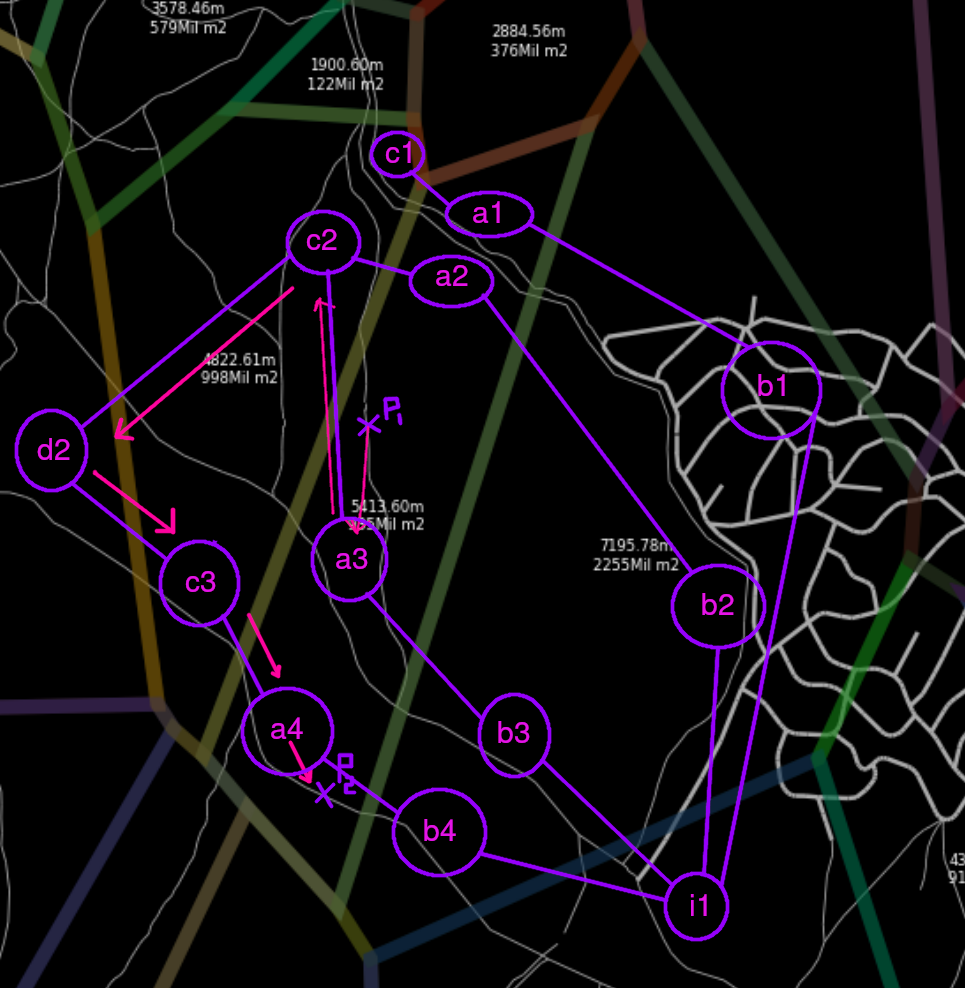
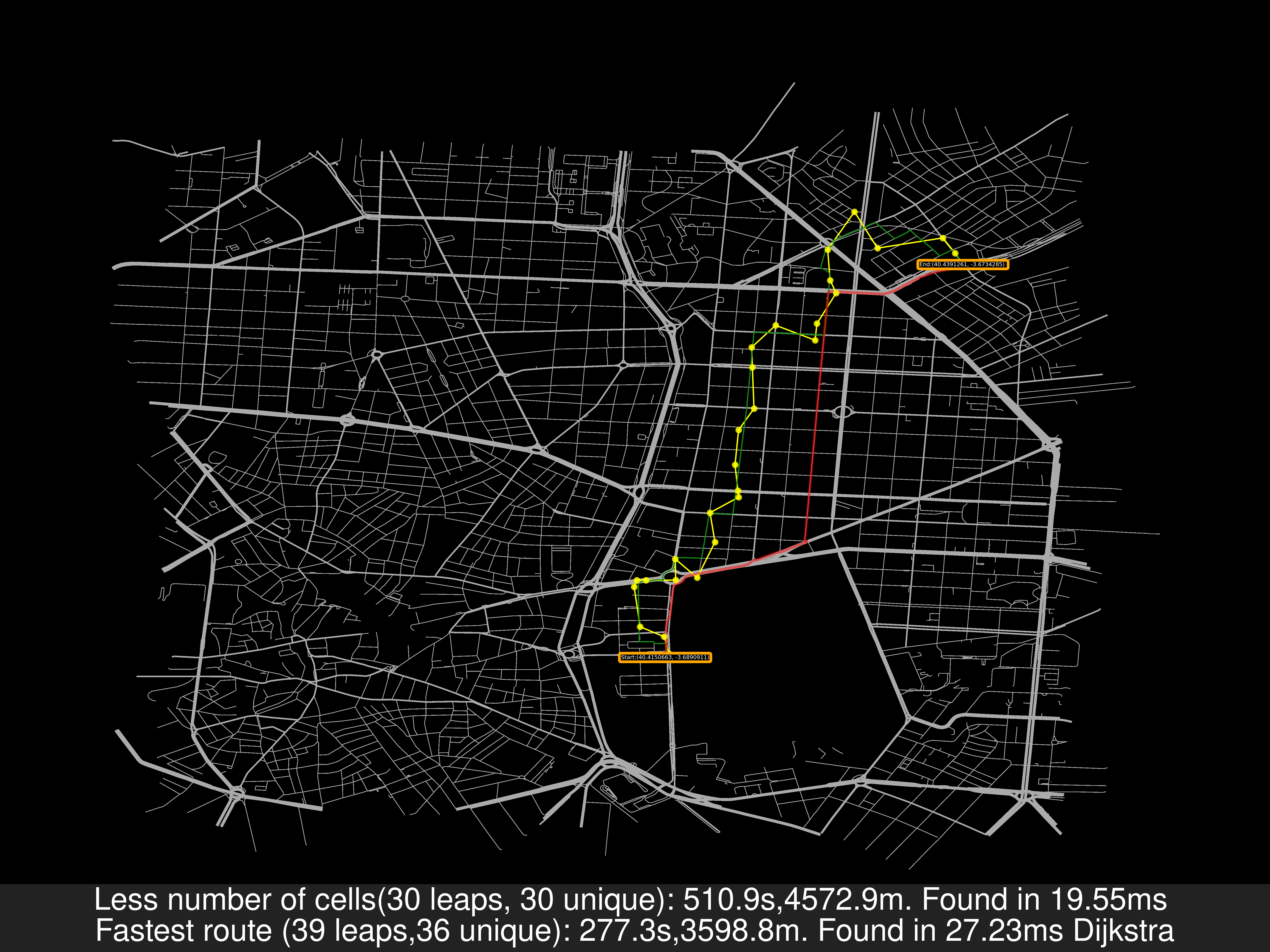
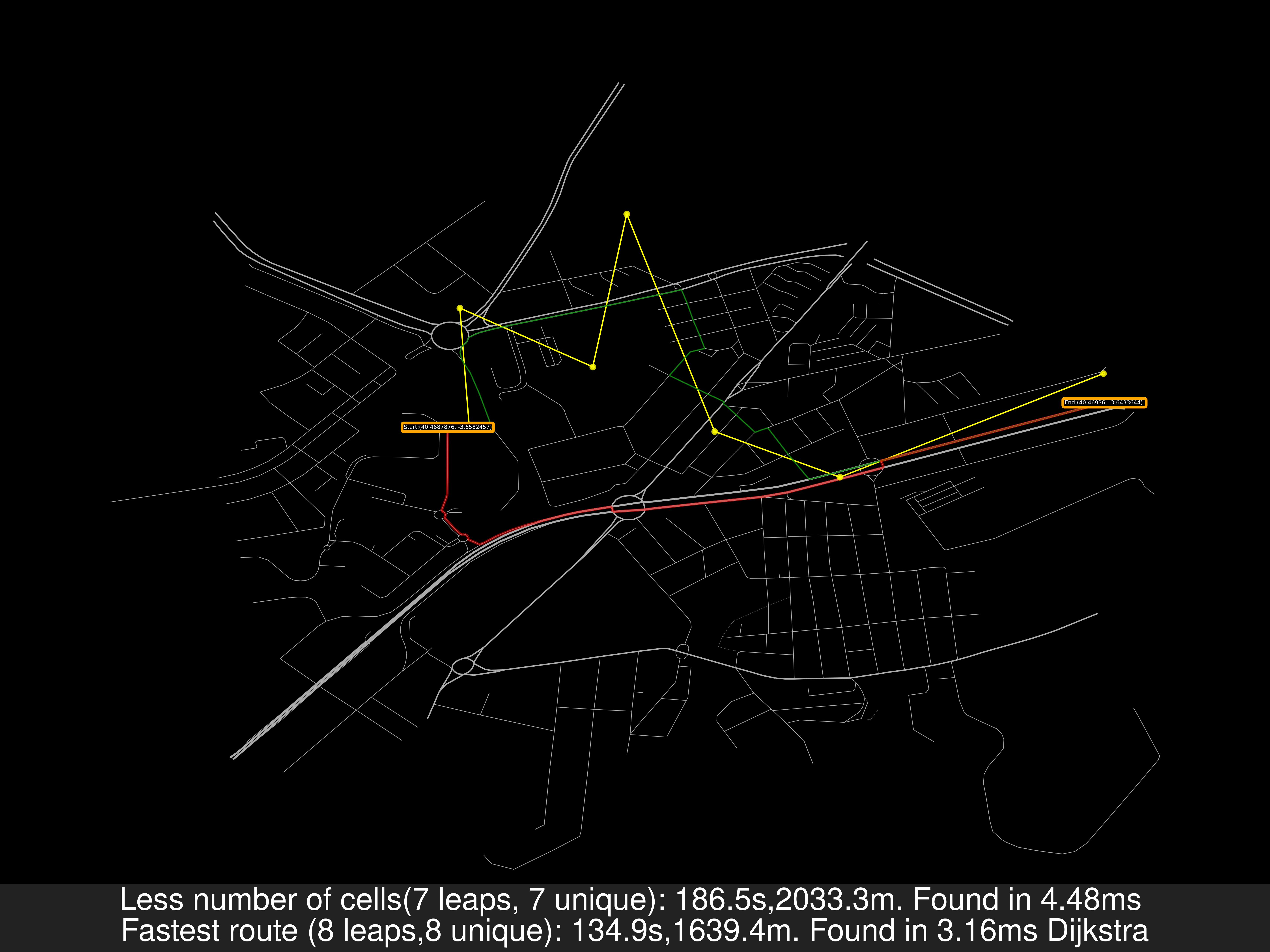
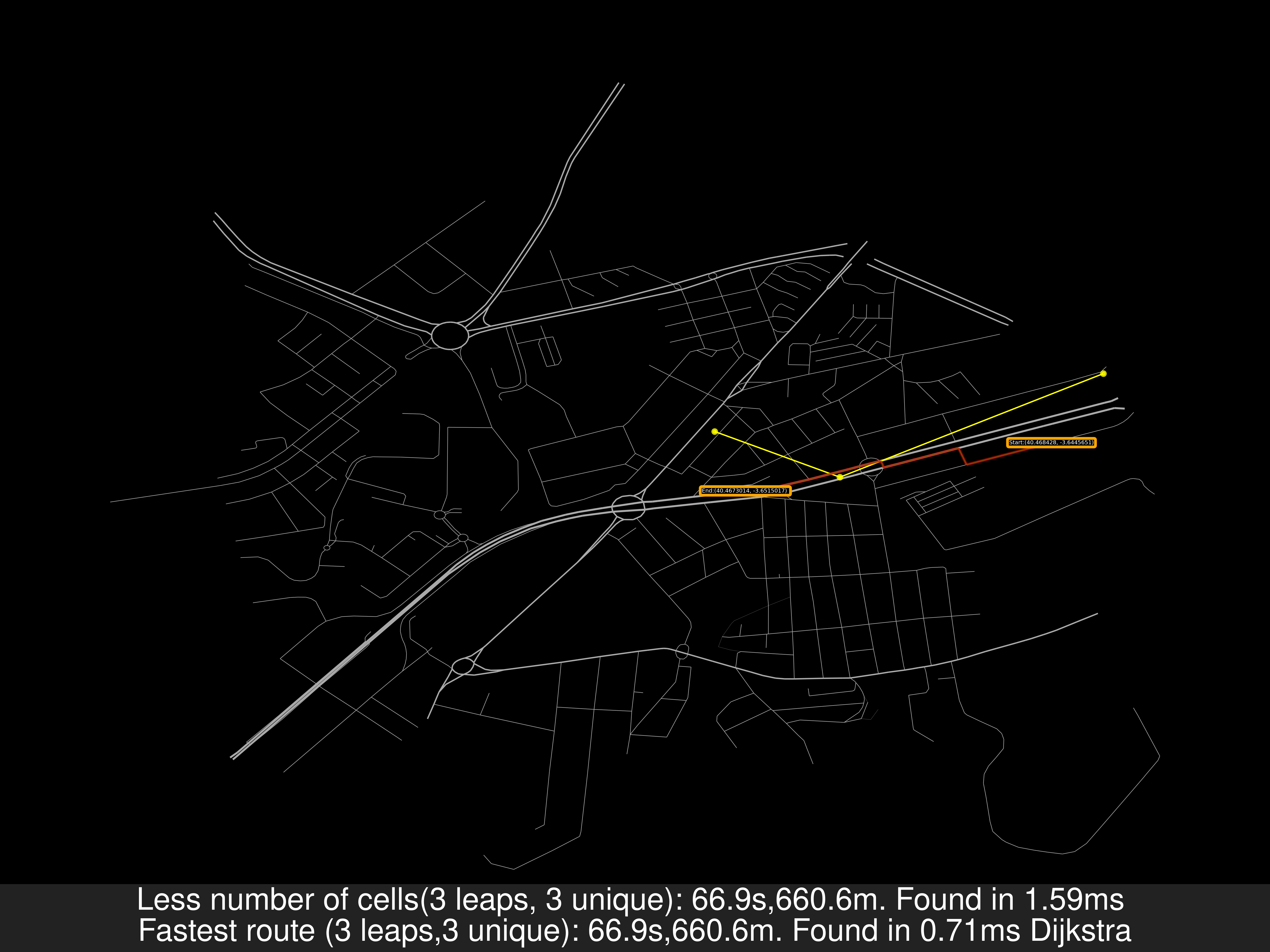
- We join the set of roads and perform the searching algorithm (i.e. A*) and we obtain the shortest path in road, painted in green.
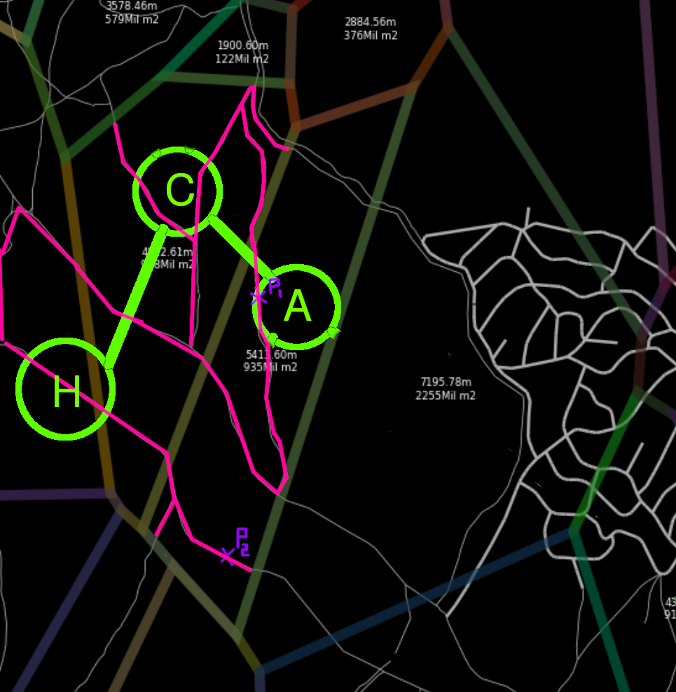
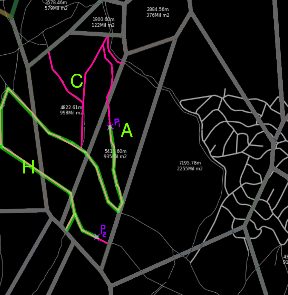
In step 3, using a shortest path solving we are guaranteeing that the resuling path uses the less ammount of jumps between cells, this is not guaranteed if we solve the shortest path only having into consideration the road network.
How different is the new algorithm?
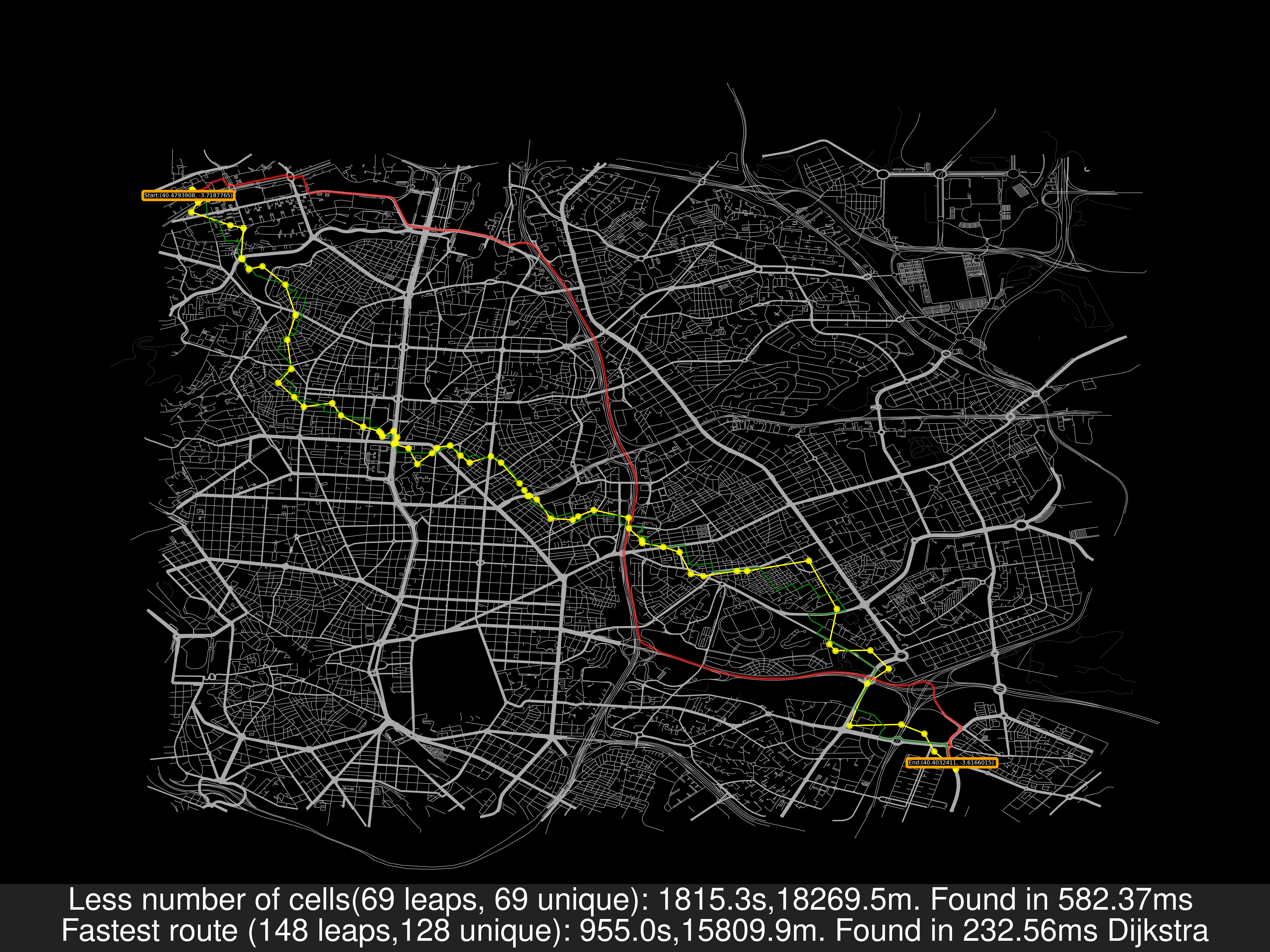
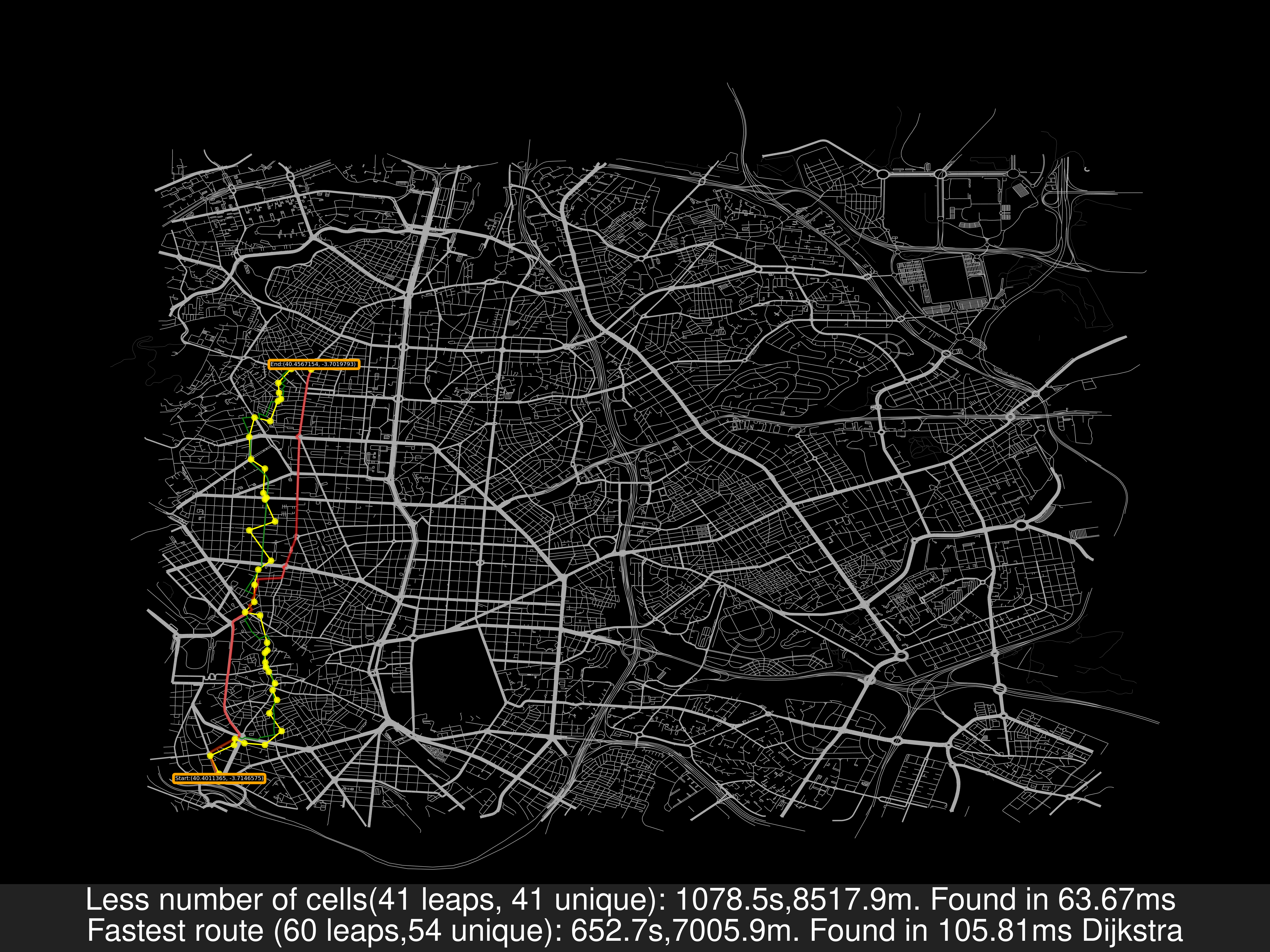
Because this algorithms seeks for the less ammount of jumps between cells. We have to compare what’s the tradeoff against the shortest path by road (ignoring cells). Simulating shortest path for two random points:
| distances | nsamples | Cell Hops New/Old [%] | Cells Used New/Old | Travel Time New/Old | max TT New/Old | Time of Compute New/Old | max ToC New/Old | CellSeconds |
|---|---|---|---|---|---|---|---|---|
| 0 < 1km | 1178 | 95.02 | 1.01 | 1.15 | 26.19 | 3.66 | 386.61 | 1.33 |
| 1 km <= 2km | 1766 | 86.21 | 0.92 | 1.24 | 10.95 | 2.26 | 54.30 | 1.23 |
| 2 km <= 3km | 1270 | 77.43 | 0.83 | 1.36 | 8.90 | 1.31 | 66.31 | 1.19 |
| 3 km <= 5km | 2061 | 68.35 | 0.74 | 1.46 | 7.55 | 1.17 | 80.62 | 1.10 |
| 5 km <= 10km | 2595 | 60.47 | 0.67 | 1.60 | 3.99 | 1.22 | 52.98 | 1.07 |
| 10 km <= 15km | 1083 | 54.83 | 0.60 | 1.62 | 3.75 | 1.58 | 86.20 | 0.94 |
| 15km or more | 899 | 50.09 | 0.53 | 1.39 | 2.57 | 1.91 | 40.59 | 0.71 |
Fields: The stats New/Old are the division between results with this algorithm and A* _Although in the pictures there’s a label Dijkstra, it’s A*
- Distances: Distance of the path A* between points
P1andP2 - nsamples: Number of samples per distance range
- Cell Hops: Times the path changes from one cell to another (i.e.
A1,A2,A1,A3,A2→ 4 hops) - Cells Used: Unique set of Cell Hops (i.e.
A1,A2,A3→ 3 cells used) - Travel Time: Total travel time of the path
- max TT: maximum travel time, “worst case”
- Time of Compute: Time needed for finding the shortest path:
- Old: Only A* into consideration
- New: Time needed for the path in the cell graph and the in the subset road graph
- CellSeconds: Metric inspired on the energy unit [KWh]: (NewCellsUsed*NewTravelTime)/(OldCellsUsed*OldTravelTime) i.e. 4 cells for 300 seconds = 1200 Cs ⇔ 16 cells for 75 seconds = 1200 Cs Few example of zones:
- Madrid Hortaleza SanBlas Tetuan :
| distances | nsamples | Cell Hops New/Old [%] | Cells Used New/Old | Travel Time New/Old | max TT New/Old | Time of Compute New/Old | max ToC New/Old | CellSeconds |
|---|---|---|---|---|---|---|---|---|
| 0 < 1km | 25 | 93.14 | 0.99 | 1.50 | 9.36 | 6.68 | 112.58 | 1.55 |
| 1 km <= 2km | 97 | 92.45 | 0.99 | 1.66 | 10.95 | 2.49 | 38.65 | 2.54 |
| 2 km <= 3km | 128 | 79.58 | 0.85 | 1.57 | 8.11 | 1.10 | 14.28 | 1.49 |
| 3 km <= 5km | 386 | 68.57 | 0.75 | 1.61 | 7.55 | 1.02 | 16.09 | 1.29 |
| 5 km <= 10km | 1034 | 56.71 | 0.64 | 1.71 | 3.69 | 1.06 | 11.25 | 1.10 |
| 10 km <= 15km | 433 | 49.14 | 0.56 | 1.77 | 3.04 | 1.52 | 4.54 | 1.01 |
| 15km or more | 33 | 46.01 | 0.54 | 1.86 | 2.46 | 2.13 | 4.61 | 1.01 |
- Madrid Centro:
| distances | nsamples | Cell Hops New/Old [%] | Cells Used New/Old | Travel Time New/Old | max TT New/Old | Time of Compute New/Old | max ToC New/Old | CellSeconds |
|---|---|---|---|---|---|---|---|---|
| 0 < 1km | 84 | 91.43 | 1.02 | 1.52 | 26.19 | 6.65 | 386.61 | 3.85 |
| 1 km <= 2km | 210 | 82.64 | 0.89 | 1.65 | 9.58 | 1.66 | 54.30 | 1.73 |
| 2 km <= 3km | 331 | 77.52 | 0.85 | 1.65 | 8.90 | 1.23 | 66.31 | 1.57 |
| 3 km <= 5km | 762 | 65.40 | 0.72 | 1.58 | 5.83 | 1.11 | 41.10 | 1.17 |
| 5 km <= 10km | 878 | 58.66 | 0.66 | 1.65 | 3.02 | 1.27 | 32.34 | 1.11 |
| 10 km <= 15km | 22 | 50.87 | 0.57 | 1.56 | 2.03 | 1.47 | 3.24 | 0.96 |
- Alcobendas:
| distances | nsamples | Cell Hops New/Old [%] | Cells Used New/Old | Travel Time New/Old | max TT New/Old | Time of Compute New/Old | max ToC New/Old | CellSeconds |
|---|---|---|---|---|---|---|---|---|
| 0 < 1km | 164 | 90.97 | 0.94 | 1.10 | 2.22 | 3.26 | 39.94 | 1.01 |
| 1 km <= 2km | 447 | 82.88 | 0.87 | 1.20 | 7.24 | 1.75 | 44.99 | 1.05 |
| 2 km <= 3km | 604 | 76.30 | 0.80 | 1.24 | 2.67 | 1.08 | 8.66 | 0.99 |
| 3 km <= 5km | 719 | 69.71 | 0.74 | 1.29 | 3.73 | 1.29 | 80.62 | 0.95 |
| 5 km <= 10km | 220 | 59.73 | 0.64 | 1.31 | 2.25 | 1.45 | 7.31 | 0.83 |

- Alcobendas Small:
| distances | nsamples | Cell Hops New/Old [%] | Cells Used New/Old | Travel Time New/Old | max TT New/Old | Time of Compute New/Old | max ToC New/Old | CellSeconds |
|---|---|---|---|---|---|---|---|---|
| 0 < 1km | 887 | 96.33 | 1.02 | 1.11 | 5.07 | 3.38 | 60.09 | 1.15 |
| 1 km <= 2km | 951 | 87.60 | 0.94 | 1.12 | 2.93 | 2.64 | 51.18 | 1.07 |
| 2 km <= 3km | 132 | 78.12 | 0.86 | 1.08 | 1.57 | 2.76 | 12.46 | 0.95 |
| 3 km <= 5km | 7 | 76.47 | 0.84 | 0.94 | 1.12 | 2.68 | 3.39 | 0.89 |

- Alcobendas TresCantos FuentedelFresno:
| distances | nsamples | Cell Hops New/Old [%] | Cells Used New/Old | Travel Time New/Old | max TT New/Old | Time of Compute New/Old | max ToC New/Old | CellSeconds |
|---|---|---|---|---|---|---|---|---|
| 0 < 1km | 18 | 86.67 | 0.93 | 1.16 | 1.98 | 3.12 | 8.69 | 1.06 |
| 1 km <= 2km | 61 | 91.43 | 0.96 | 1.15 | 3.58 | 1.73 | 13.17 | 1.14 |
| 2 km <= 3km | 75 | 81.24 | 0.87 | 1.25 | 2.88 | 1.19 | 8.09 | 1.10 |
| 3 km <= 5km | 187 | 74.38 | 0.79 | 1.31 | 4.10 | 1.21 | 8.71 | 1.03 |
| 5 km <= 10km | 463 | 72.67 | 0.77 | 1.41 | 3.99 | 1.37 | 52.98 | 1.07 |
| 10 km <= 15km | 628 | 58.90 | 0.62 | 1.51 | 3.75 | 1.63 | 86.20 | 0.90 |
| 15km or more | 866 | 50.25 | 0.53 | 1.37 | 2.57 | 1.90 | 40.59 | 0.70 |
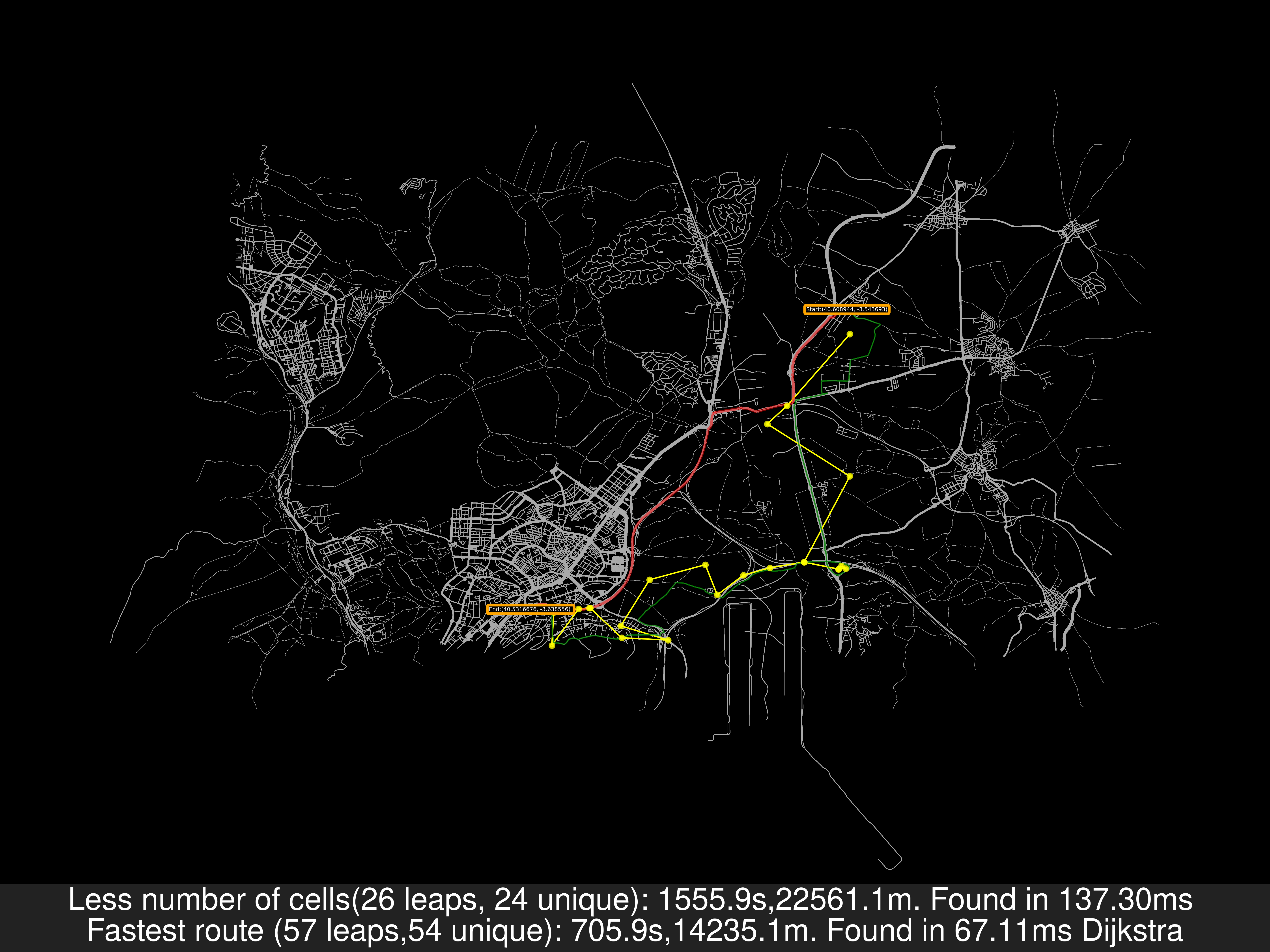
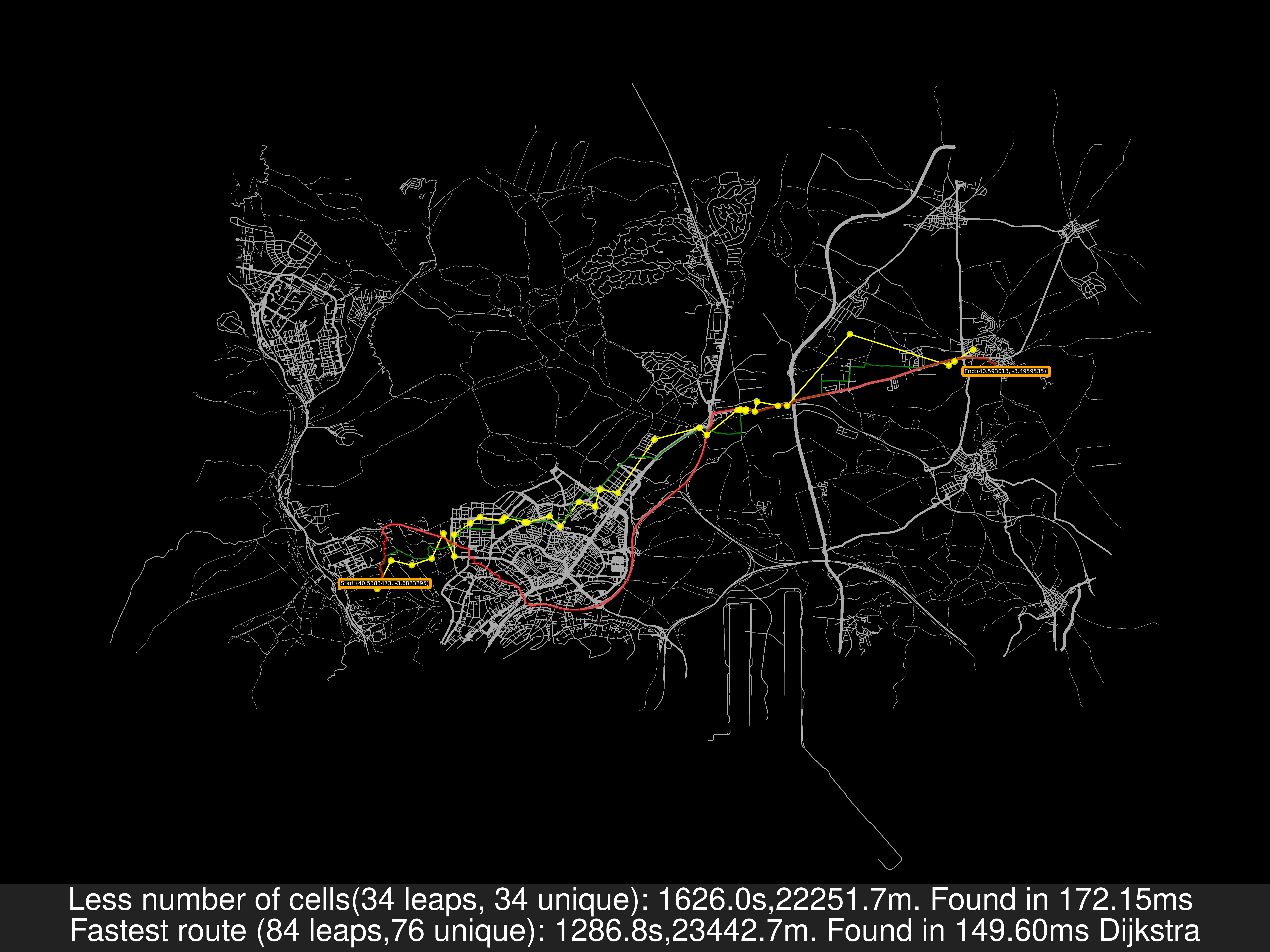
As a remainder: In the previous image, the travel distance is greater in the Less cells case but the travel time is smaller. That’s because for the road’s speed I’ve used uber movement data