Last Modified: 2023-Jun-29
INTRO Roadmap
Índice
Objective
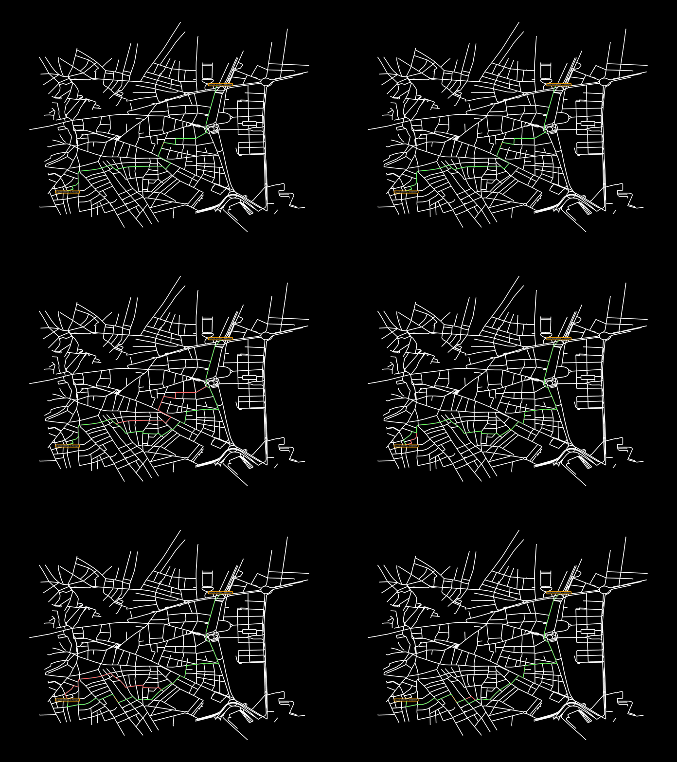
To Develop a Python environment, based on the NetworkX library, in order to study route planning algorithms in a scenario of remote driving with real environments. The overall goal is to minimize the number of cells required to perform a remote drive, in order to maximize the number of hypothetical cars/travels that can be performed at the same time.
The main milestones are:
- Roads: Obtain realistic road data
- Speed data
- Graph representation: of the roads
- Base Stations: Obtain realistic data of base stations’ positions]
- Create a graph of base stations
- Find the shortest path between two base stations
- Implement a 2 layer routing algorithm
- Analyze the results


Steps
Roads
Using Overpass, OSM’s API, we can obtain data of the roads in a certain area, for example, the center of Madrid.
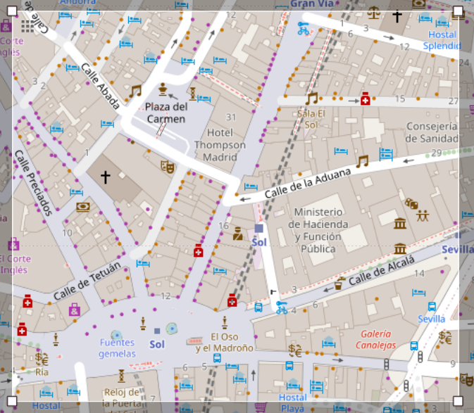
Overpass’s queries have their own language (Overpass QL) somewhat like SQL, but for interacting with OSM’s API. This can be easily learned by using the Overpass Turbo web interface and following the ldodds’ tutorial.
As a summary, some of the main objects in the query are way and node, which are the main objects to define roads and intersections, respectively.
Defining a bounding box bbox or a center and radious around, we can obtain the data of the roads in that area. Further filtering can be accomplished by using tags, due to the fact that the data is user generated, the quality of the data can vary, hence roads with similar characteristics can differ in the tags they have. Luckily I some tags from Project-OSRM and added another tags that appear in the roads I was interested in.
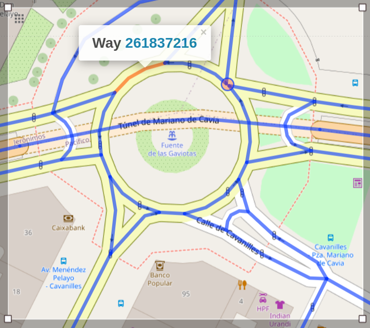
Example of filtered data and non filtered data
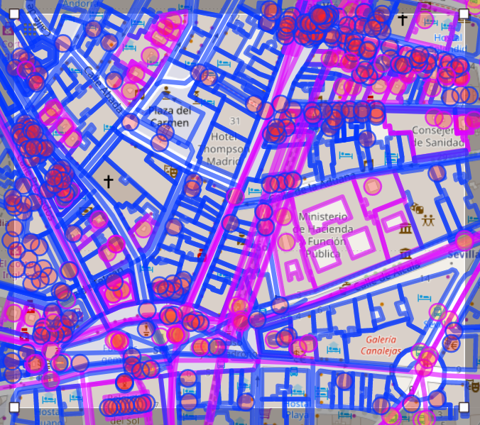

Note: There are tags like direction, lanes, maxspeed, name, oneway, surface, width and many more.
Characterizing roads’ congestion
From UberMovement we can obtain data of the roads’ congestion, understood as the average speed of the cars that pass through that road. This data lists roads’s average speed per hour, per day, per month, per year. Although not every road has data for every hour, it’s still a good approximation of the road’s congestion.
| Field | Description |
|---|---|
| year | - |
| month | - |
| day | - |
| hour | - |
| osm_way_id | UID of the road section (way) in OSM |
| osm_start_node_id | UID of the start node of the way |
| osm_end_node_id | UID of the end node of the way |
| speed_kph_mean | - |
| speed_kph_stddev | - |
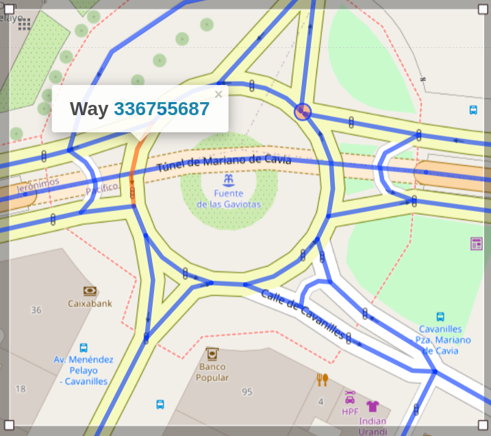
I will just use the mean speed and put the data into an SQL DB.
Graph representation
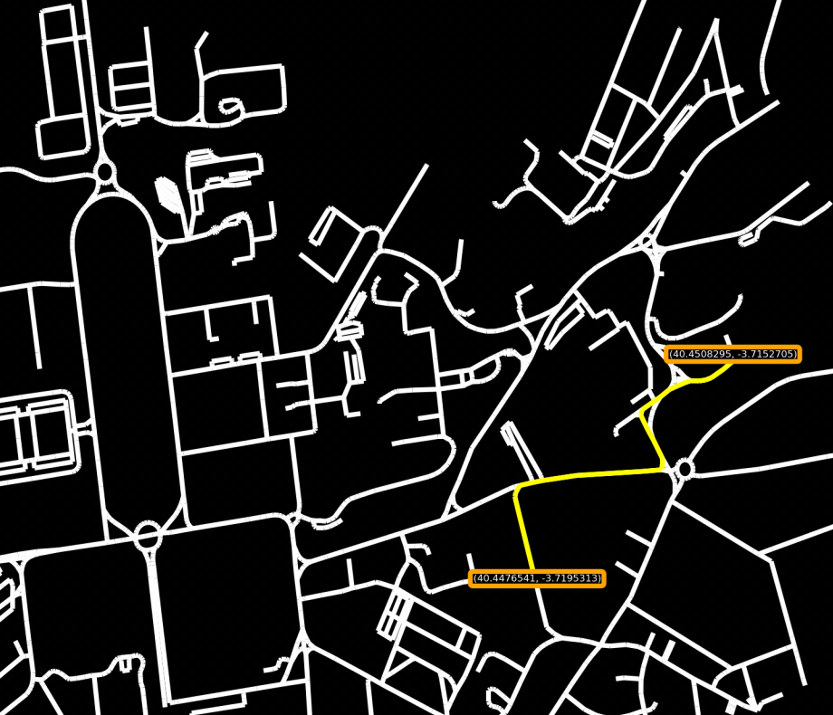
For network analysis, we can represent the roads as a graph, where the nodes are the intersections and the edges are the roads. To treat this data in graph form, it’s loaded into a Networkx graph. NetworkX is a library that facilitates the creation, manipulation, and study of the structure, dynamics, and functions of complex networks. I will use Dijkstra and A* algorithms to find the shortest path between two nodes.
import networkx as nx
Graph=nx.Graph()
ways_nodes=queryOSM(lat,long)
Graph.add_edges_from(ways_nodes)
...
ShortestPath=nx.dijkstra_path(Graph,node_start,node_end) # Array de nodos
...
paint(Graph)
paint(ShortestPath)
Joining uber and osm data
In Networkx, the vertices or edges are added as 3-tuples (u,v,data), data is a dictionary with arbitrary information, which we want to access later, for example, during the search for the shortest path or when representing paint the graph. In data['speed'] the “current” speed is saved:
import networkx as nx
Graph=nx.Graph()
ways_nodes=queryOSM(lat,long)
Graph.add_edges_from(ways_nodes) #  Roards as gaphs
ubermv.updatespeed(Graph,hora=9,dia=Friday) # Update the speed of the roads
...
ShortestPath=nx.dijkstra_path(Graph,node_start,node_end) # Array de nodos
...
paint(Graph)
paint(ShortestPath)
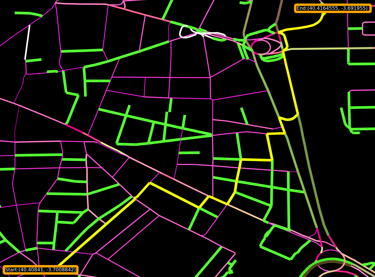
Some representations
-
Roads with their’s widths and colors as their average speed (greener and thicker is faster) and the shortest path in yellow.
-
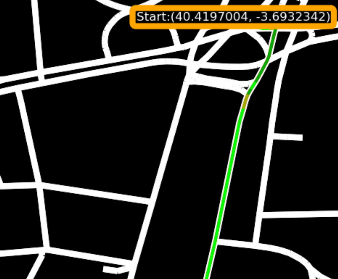
Speeds in the shortest path.
-
Gif of the shortest path (Dijkstra) throughout the day
